CALCULATE PI USING MONTECARLO SIMULATION – PHASE III – aka "Multicarlo"


Introduction

After Phase II, we discovered that Numpy wasn’t going to help. Also, getting a half way decent approximation of Pi was going to take millions of paths / attempts. So on a slimmed down calculation where the [x,y] position of each random try was not kept, what could be done to make this as quick and accurate as possible?

Multi-Processing?

Can I use the 16 Cores on my machine to go 16X faster? Am I being naiive here? If I am, how and what is the most that can be done? I would like to see if the infamous G.I.L will Get me Into Logjam or not.

First Attempt [Disaster]

from multiprocessing import Pool
import os

num_cpus = os.cpu_count()
print('Num of CPUS: {}'.format(num_cpus))

try:
    pool = Pool(num_cpus) # on 8 processors
    data_outputs = pool.map(calc_pi_quick, [10])
    print (data_outputs)
finally: # To make sure processes are closed in the end, even if errors happen
    pool.close()
    pool.join()

Disappointingly, not only is it not any quicker; in fact, doesn’t finish running AT ALL.

Awkward, lets look at why that is happening first?

  • I quite like Medium Articles and this one seems to hit the spot.
  • Also this from StackOverflow

Second Attempt

from random import random

def calc_pi_quick(num_attempts: int) -> float:
    from random import random

    inside = 0

    for _ in range(num_attempts):
        x = random()
        y = random()

        if x ** 2 + y ** 2 <= 1:
            inside += 1

    return 4 * inside / num_attempts


def multi_calc_pi(num_attempts: int, verbose=False) -> float:
    from multiprocessing import Pool
    from random import random
    import os
    from statistics import mean

    # lets leave one spare for OS related things so everything doesn't freeze up
    num_cpus = os.cpu_count() - 1
    # print('Num of CPUS: {}'.format(num_cpus))

    try:
        attempts_to_try_in_process = int(num_attempts / num_cpus)
        pool = Pool(num_cpus)
        # what I am trying to do here is get the calc happening over n-1 Cpus each with an even
        # split of the num_attempts. i.e. 150 attempts over 15 CPU will lead to 10 each then the mean avg
        # of the returned list being returned.
        data_outputs = pool.map(calc_pi_quick, [attempts_to_try_in_process] * num_cpus)
        return mean(data_outputs)
    finally:  # To make sure processes are closed in the end, even if errors happen
        pool.close()
        pool.join()

To get multiprocessing to work on Jupyter Notebooks and Windows 10, I had to save this code to a different file to be called from the Jupyter Notebook, and executed within __main__. However once I did, this did lead to a significant performance increase.

Collect the Stats

import calcpi
from timeit import default_timer as timer
from datetime import timedelta
import matplotlib.pyplot as plt

if __name__ == '__main__':
    
    num_attempts = [50, 500, 5_000, 50_000, 500_000, 5_000_000, 50_000_000]
    multi_timings = []
    single_timings = []
    
    for x in num_attempts:
    
        start = timer()
        multi_pi = calcpi.multi_calc_pi(x)
        end = timer()  
        multi_timings.append((end-start))
        print("MultiCarlo Pi: {}: {} took {}".format(multi_pi, x, timedelta(seconds=end-start)))

        start = timer()    
        pi = calcpi.calc_pi_quick(x)
        end = timer()
        single_timings.append((end-start))
        print("MonteCarlo Pi: {}: {} took {}".format(pi, x, timedelta(seconds=end-start)))

    plt.plot(num_attempts, multi_timings)
    plt.plot(num_attempts, single_timings)

    plt.show()

Display the stats in a more meaningful way

import plotly.graph_objects as go

import numpy as np

# lets pretty this up so the axis label is more readable
x_axis = ['{:,}'.format(x) for x in num_attempts]

fig = go.Figure(data=[
    go.Bar(name='Multi Process', x=x_axis, y=multi_timings),
    go.Bar(name='Single Process', x=x_axis, y=single_timings)
])
# Change the bar mode
fig.update_layout(xaxis_type='category',barmode='group')
fig.show()
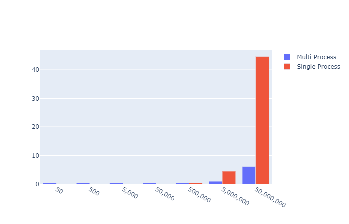
Single vs Multiprocessing for increasing simulation size

Early on in the exponentially increasing simulation size, the overhead of creating the Pool, asking the os for CPU count the splitting the attempts up to the pool seemed to result in a floor of 0.4s. However, at that level the Pi value returned was nonsense anyway. So I think the overhead for any reasonable approximation of Pi is worth the set up cost in this case.

Baby, can I get your Numba?

Can we go even further? I think we could give Numba a try.

After some research and reading around the internet for a day or so while avoiding Covid-19 I found out it is incredibly simple.

4 little chars that change everything. @jit

from random import random
from numba import njit, jit

@jit
def calc_pi_numba(num_attempts: int) -> float:
    inside = 0

    for _ in range(num_attempts):
        x = random()
        y = random()

        if x ** 2 + y ** 2 <= 1:
            inside += 1

    return 4 * inside / num_attempts

That is it. Just one import and one teensy little decorator and we are away. How does this stack up agianst my mighty multi monte carlo from earlier though?

Lets get some timings

import calcpi
from timeit import default_timer as timer
from datetime import timedelta
import matplotlib.pyplot as plt
import plotly.graph_objects as go

if __name__ == '__main__':
    
    num_attempts = [50, 500, 5_000, 50_000, 500_000, 5_000_000, 50_000_000]
    function_list = [calcpi.calc_pi_quick, calcpi.calc_pi_numba, calcpi.multi_calc_pi]
    results_dict = {}

    for func in function_list:

        timings = []
        
        for x in num_attempts:
        
            start = timer()
            pi = func(x)
            end = timer()  
            timings.append((end-start))
            # print("{} => Pi: {} Attempts: {} Time: {}".format(func.__name__, pi, x, timedelta(seconds=end-start)))

        results_dict[func.__name__] = timings
    
    go_data = []
    # lets pretty this up so the axis label is more readable
    x_axis = ['{:,}'.format(x) for x in num_attempts]
    
    for func in function_list:
    
        plt.plot(num_attempts, results_dict[func.__name__])
        
        go_data.append(go.Bar(name=func.__name__, x=x_axis, y=results_dict[func.__name__]))

    plt.show()

    fig = go.Figure(data=go_data)
    # Change the bar mode
    fig.update_layout(xaxis_type='category',barmode='group')
    fig.show()
        

Results visulisation
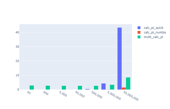
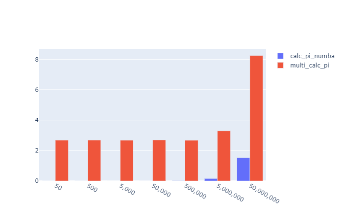
X: Attempts Y: Seconds to run

Oh… it absolutely smashes it.

Out of the park for

  • Speed
  • Readability
  • Implementation simplicity

CALCULATE PI USING MONTECARLO SIMULATION – PHASE II


Context

Carrying on from Phase I, I wanted to see how I could take the initial answer and make it more efficient. The first port of call then is… how expensive is it at the moment. Will any changes I make have a significant impact on that baseline.

timeit

I dont think using %%timeit as an ipython coding secret on the cell will cut the mustard, but we shall see. I would like to be able to single out code sections for timing too.

Calc Pi Unoptimised

def calc_pi(num_attempts, display_plot=False):

    import matplotlib
    import matplotlib.pyplot as plt
    from random import random
    
    inside = 0

    x_inside = []
    y_inside = []
    x_outside = []
    y_outside = []

    for _ in range(num_attempts):
        x = random()
        y = random()
        if x**2+y**2 <= 1:
            inside += 1
            x_inside.append(x)
            y_inside.append(y)
        else:
            x_outside.append(x)
            y_outside.append(y)

    pi = 4*inside/num_attempts
    
    if display_plot:
        fig, ax = plt.subplots()
        ax.set_aspect('equal')
        ax.scatter(x_inside, y_inside, color='g')
        ax.scatter(x_outside, y_outside, color='r')

    return pi

Calc Pi Quick (Version 1)

Quick Python only changes, remove array recording and if we never plan to plot remove the if statement

def calc_pi_quick(num_attempts: int):

    inside = 0

    for _ in range(num_attempts):
        x = random()
        y = random()
        if x**2+y**2 <= 1:
            inside += 1

    return 4*inside/num_attempts

Initial comparison

from timeit import default_timer as timer
from datetime import timedelta

start = timer()
calc_pi(50000000, True)
end = timer()
print(timedelta(seconds=end-start))

start = timer()
calc_pi(50000000, False)
end = timer()
print(timedelta(seconds=end-start))

start = timer()
calc_pi_quick(50000000)
end = timer()
print(timedelta(seconds=end-start))

Output

calc_pi with plotly display time: 0:00:08.318734 
calc_pi no display time: 0:00:00.625193 
calc_pi_quick time: 0:00:00.470770

We start to see there are some decent performance benefits. Lets check if these are linear or not. However to see some really decent improvements I think we can start to think about threading perhaps? Also if we still wanted to record the hit and miss positions, would numpy be quick enough that we can keep this data without a significant performance hit?

Numpy Optimisation Attempts

Spoiler Alert… my first attempt was absolutely terrible. However, in a way that’s great news. I now know what not to do with numpy on a non trivial problem, and now so do you.

def calc_pi_numpi_bad(num_attempts):
    
    import numpy as np
    import matplotlib
    import matplotlib.pyplot as plt
    from random import random
    
    inside = 0

    x_inside = np.array([])
    y_inside = np.array([])
    x_outside = np.array([])
    y_outside = np.array([])

    for _ in range(num_attempts):
        x = random()
        y = random()
        if x**2+y**2 <= 1:
            inside += 1
            x_inside = np.append(x_inside, x)
            y_inside = np.append(y_inside, y)
        else:
            x_outside = np.append(x_outside, x)
            y_outside = np.append(y_outside, y)

    pi = 4*inside/num_attempts

    return pi

How bad? Well lets see…

def measure_performance_verbose(num_attempts: int) -> None:

    from timeit import default_timer as timer
    from datetime import timedelta

    start = timer()
    calc_pi(num_attempts, False)
    end = timer()
    time_taken = end-start
    print('calc_pi time: {}'.format(timedelta(seconds=time_taken)))

    start = timer()
    calc_pi_quick(num_attempts)
    end = timer()
    quick_time_taken = end-start
    print('calc_pi_quick time: {}'.format(timedelta(seconds=quick_time_taken)))

    percentage_improvement = quick_time_taken / time_taken * 100
    
    print('Precentage improvement: {}'.format(percentage_improvement))

    start = timer()
    calc_pi_numpi(num_attempts)
    end = timer()
    numpi_time_taken = end-start
    print('calc_pi_numpi time: {}'.format(timedelta(seconds=numpi_time_taken)))
    
    start = timer()
    calc_pi_numpi_bad(num_attempts)
    end = timer()
    numpi_bad_time_taken = end-start
    print('calc_pi_numpi_bad time: {}'.format(timedelta(seconds=numpi_bad_time_taken)))
    
    
measure_performance_verbose(500_000)
calc_pi time: 0:00:00.636658
calc_pi_quick time: 0:00:00.462309
Precentage improvement: 72.6149660351135
calc_pi_numpi time: 0:00:00.616958
calc_pi_numpi_bad time: 0:12:52.784511

Whoa, what just happened there. It takes TWELVE seconds to run for 500,000 attempts. That is atrocious.

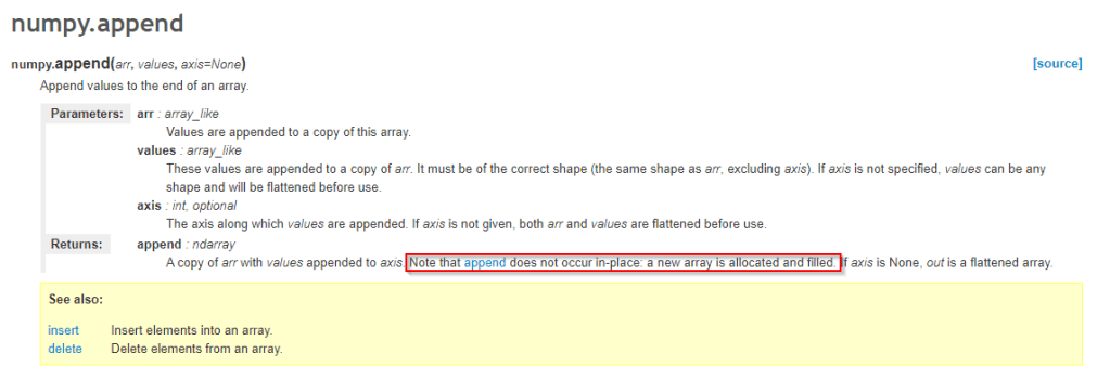
Lets look at the documentation for this function.

Ahh, that explains it. Every append copies the existing array into a new one. I did not know that, shame on me. I have always used np arrays as data converted from pandas or existing python lists, not created and appended to them on the fly.

However, we can fix it by pre-allocating the mem to the max num required and then mask the results if zero in plotly.

def calc_pi_numpi(num_attempts, display_plot=False, display_masked_plot=False):
    
    import numpy as np
    import matplotlib
    import matplotlib.pyplot as plt
    from random import random
    
    inside = 0

    x_inside = np.zeros(num_attempts)
    y_inside = np.zeros(num_attempts)
    x_outside = np.zeros(num_attempts)
    y_outside = np.zeros(num_attempts)

    for i in range(num_attempts):
        x = random()
        y = random()
        if x**2+y**2 <= 1:
            inside += 1
            x_inside[i] = x
            y_inside[i] = y
        else:
            x_outside[i] = x
            y_outside[i] = y

    if display_masked_plot:
        
        fig, ax = plt.subplots()
        ax.set_aspect('equal')
        ax.scatter(np.ma.masked_equal(x_inside,0), np.ma.masked_equal(y_inside,0), color='g')
        ax.scatter(np.ma.masked_equal(x_outside,0), np.ma.masked_equal(y_outside,0), color='r')
        
    if display_plot:
            
        x_inside2 = x_inside[x_inside !=0] 
        y_inside2 = y_inside[y_inside !=0]
        x_outside2 = x_outside[x_outside !=0]
        y_outside2 = y_outside[y_outside !=0]

        fig, ax = plt.subplots()
        ax.set_aspect('equal')
        ax.scatter(x_inside2, y_inside2, color='g')
        ax.scatter(x_outside2, y_outside2, color='r')

    pi = 4*inside/num_attempts

    return pi

There are two booleans so that we can test that both work.

calc_pi_numpi(256, True, True)
masked


numpy zero removal
start = timer()
calc_pi_numpi(500_000, True, False)
end = timer()
time_taken = end-start
print('calc_pi normal display time: {}'.format(timedelta(seconds=time_taken)))

start = timer()
calc_pi_numpi(500_000, False, True)
end = timer()
time_taken = end-start
print('calc_pi masked display time: {}'.format(timedelta(seconds=time_taken)))
calc_pi normal display time: 0:00:02.356013
calc_pi masked display time: 0:00:04.012019

Much much better.

start = timer()
calc_pi_numpi(500_000, False, False)
end = timer()
time_taken = end-start
print('calc_pi no display time: {}'.format(timedelta(seconds=time_taken)))

start = timer()
calc_pi(500_000)
end = timer()
time_taken = end-start
print('calc_pi no display time: {}'.format(timedelta(seconds=time_taken)))
calc_pi no display time: 0:00:00.622075 
calc_pi no display time: 0:00:00.655379

So… numpy doesn’t make things better, but used correctly, doesn’t make things any worse. So this is a dead end. Also we don’t want to plot for the numbers higher than a million as it looks to the human eye to be , a complete quarter circle. in plotly anyway so we dont need to store large amounts of array data anyway

While I am here I wanted to utilise the “functions are first class objects” paradigm in python. I have hinted at it by showing the initial fuction as _verbose but its much cleaner to call that same code within a functor ( of sorts ) loop as below.

def measure_performance(num_attempts: int) -> None:

    from timeit import default_timer as timer
    from datetime import timedelta
    
    funcs_to_call = [calc_pi, calc_pi_quick, calc_pi_numpi, calc_pi_numpi_bad]
    
    for func in funcs_to_call:
        start = timer()
        calc_pi(num_attempts, False)
        end = timer()
        time_taken = end-start
        print('{} time: {}'.format(func.__name__, timedelta(seconds=time_taken)))
    
measure_performance(50000)

In Phase III -> aka PiMultiCarlo I want to loo at what we can do locally on a decent multi core machine to get some decent speed improvements for only calculating the number only, not storing the guesses.

Follow-up

For Part III : CALCULATE PI USING MONTECARLO SIMULATION – PHASE III – aka “Multicarlo”

Google Music Takeout – Track Data


I always find working through a text book that it gets quite dry, and I struggle to maintain interest as the project or subject matter is too esoteric.

So, armed with a little python, StackOverflow and a search engine, I decided to see what I could do with my own data.

Photo by Clem Onojeghuo on Unsplash

What have I been listening to for the last three or four years?

Google allows users access to all their past data, and as a long time user of Google Music I wondered what the oversight on all this would be. Unlike Spotify, there doesn’t seem to be any scope for introspection into musical history or taste, which strikes me as odd. I guess Google is more about harvesting and selling the data, whereas Spotify realises that showing insight into their users activity and taste helps drive traffic and engagement levels.

Google Takeout Track dataset structure

unzipped takeout tracks, highlighting the weirder filenames

Seriously? A gazillion CSV files? Well… 14,646. That’s the best they can do? However, I then thought, hang on… combining multiple CSV files and cleaning up rubbish data in the dataset is the exact sort of basic data science 101 that every project has. Bring it on.

Track csv file combination

Python to combine the .csv files, lifted from my Jupyter Notebook

import os

# change as required, obviously
directory = '/takeout_data/Google Play Music/Tracks'

csv_files = []

for root,dirs,files in os.walk(directory):
    for file in files:
       if file.endswith(".csv"):
            csv_files.append(directory + "\\" + file)
            
print(len(csv_files))

Now lets iterate over the files found in the selected folder, add these to a list and then concatenate these into a pandas DataFrame. I’m painfully aware that the snippet below isn’t fully “pythonic” and wouldn’t win any stack overflow plaudits. However, I am backing myself to improve this at the end and I stated this would be a warts and all development blog. As such this is a “get this working to make sure I am going in the right direction and this is a good idea overall” mode. If its working I can move on and start to make enough progress to motivate myself to keep coding on the train and before bed each night. Also to be fair this code will be run on a once per archive result basis, so doesn’t need to be hugely optimised, considering the other project time dermands.

import pandas as pd

combined_csv = []
for i, csv_file in enumerate(csv_files):
    
    x = pd.read_csv(csv_file)
     
    if not pd.isna(x['Artist'].values) and x['Play Count'][0] > 0:
         if i % 100 == 0:
            print('100th Artist found: {}. Processing {}/{}'.format(x['Artist'].values, i, total))   
    
        combined_csv.append(x)

combined_df = pd.concat(combined_csv)

Which leads to the Jupyter Notebook output:

printing the output solved my “is this working?” worries

After saving this combined .csv file I thought I would have a quick peek into the data, to check what we were actually given.

Track combination sanity check

Ok, so now I know what I’ve listened to is all in one place. I now face some issues if I want to start answering the questions I had in mind.

  • Is this data reliable, how much cleaning and transformation will be needed?
  • When did these tracks get played?
  • Where can I find the metadata for this basic track info?

I created a new Jupyter notebook in order to evaluate the data. As a cursory check I thought the tthe followong would be a good test

  • See what the song length distribution was like
  • Top Artists
  • Total Number of Songs
  • DataFrame.head() displays

Jupyter Notebook : TakeoutTrackAnalysisBlog

Sorry, something went wrong. Reload?
Sorry, we cannot display this file.
Sorry, this file is invalid so it cannot be displayed.

Further questions (for another blog post)

  • What are my most popular artists, albums and genres?
  • Do I have any dirty / unknown track data
  • What are my top 10 shortest and longest tracks

Blog at WordPress.com.

Up ↑