Guide: Finding Matrix Diagonals


As part of my “Get Ready for Senior Tech Interviews” I was looking at Hacker Rank Questions and parsing through diagnoals of a Matrix Came up.

Obviously the “I am at work, not in an interview way is to use numpy, diag” However this it about understanding the iterations instead

Guide to Finding Matrix Diagonals <!– HOW TO USE IN WORDPRESS: 1. Edit a page or post in WordPress. 2. Add a "Custom HTML" block where you want this guide to appear. 3. Copy everything from the tag below to the closing tag… 4. …and paste it directly into the Custom HTML block. 5. The guide should now render correctly on your WordPress site. –> https://cdn.tailwindcss.com body { font-family: ‘Inter’, sans-serif; } .matrix-grid { display: grid; gap: 0.5rem; } .matrix-grid.grid-3 { grid-template-columns: repeat(3, minmax(0, 1fr)); } .matrix-grid.grid-4 { grid-template-columns: repeat(4, minmax(0, 1fr)); } .matrix-cell { width: 4rem; /* 64px */ height: 4rem; /* 64px */ display: flex; align-items: center; justify-content: center; font-size: 1.25rem; /* 20px */ font-weight: 700; border-radius: 0.5rem; /* 8px */ background-color: rgb(229 231 235); color: rgb(31 41 55); transition-property: all; transition-timing-function: cubic-bezier(0.4, 0, 0.2, 1); transition-duration: 300ms; } .highlight-path { background-color: rgb(16 185 129); color: #fff; box-shadow: 0 10px 15px -3px rgb(0 0 0 / 0.1), 0 4px 6px -4px rgb(0 0 0 / 0.1); transform: scale(1.1); } .highlight-path-main { background-color: rgb(99 102 241); color: #fff; box-shadow: 0 10px 15px -3px rgb(0 0 0 / 0.1), 0 4px 6px -4px rgb(0 0 0 / 0.1); transform: scale(1.1); } .highlight-row { /* Using border instead of ring for better compatibility */ border: 4px solid rgb(56 189 248); } .highlight-col { /* Using border instead of ring for better compatibility */ border: 4px solid rgb(236 72 153); } .code-block { background-color: rgb(17 24 39); color: #fff; padding: 1rem; border-radius: 0.5rem; font-family: ui-monospace, SFMono-Regular, Menlo, Monaco, Consolas, “Liberation Mono”, “Courier New”, monospace; font-size: 0.875rem; /* 14px */ overflow-x: auto; }

Finding Matrix Diagonals

An Illustrated Guide to the Python Techniques

1. The Main Diagonal (Top-Left to Bottom-Right)

The Core Rule

For the main diagonal, the rule is the simplest. An element is on the main diagonal if its row index is equal to its column index.

row_index == column_index

The Python Code

# For the main diagonal, we use enumerate to get the index 'i'
main_diagonal = [row[i] for i, row in enumerate(matrix)]

# Or, more simply with a range
main_diagonal = [matrix[i][i] for i in range(n)]

# For matrix = [[10,20,30],[40,50,60],[70,80,90]], result is [10, 50, 90]

Interactive Example: Main Diagonal

Click through the steps. Here, n = 3 and we look for elements where row_index == col_index.

Next Step Reset

Resulting List:

[ ]

2. The Anti-Diagonal (Top-Right to Bottom-Left)

The Core Rule

For the anti-diagonal, the sum of an element’s row index and column index is always equal to n - 1.

row_index + column_index = n – 1

The Python Code

# For the anti-diagonal, we use the formula: col = n - 1 - row
anti_diagonal = [matrix[i][n - 1 - i] for i in range(n)]

# For matrix = [[10,20,30],[40,50,60],[70,80,90]], result is [30, 50, 70]

Interactive Example: Anti-Diagonal

Click through the steps. Here, n = 3, so the target index sum is n - 1 = 2.

Next Step Reset

Resulting List:

[ ]
const matrixData = [ [10, 20, 30], [40, 50, 60], [70, 80, 90] ]; const n = matrixData.length; function setupInteractiveExample(config) { let currentStep = -1; const result = []; const matrixContainer = document.getElementById(config.matrixId); const stepInfoContainer = document.getElementById(config.stepInfoId); const resultList = document.getElementById(config.resultListId); const nextStepBtn = document.getElementById(config.nextBtnId); const resetBtn = document.getElementById(config.resetBtnId); function createMatrix() { matrixContainer.innerHTML = ”; matrixData.flat().forEach((val, index) => { const cell = document.createElement(‘div’); cell.className = ‘matrix-cell’; cell.id = `${config.prefix}-cell-${Math.floor(index / n)}-${index % n}`; cell.textContent = val; matrixContainer.appendChild(cell); }); } function resetHighlights() { matrixContainer.querySelectorAll(‘.matrix-cell’).forEach(cell => { cell.classList.remove(config.highlightClass, ‘highlight-row’, ‘highlight-col’); cell.style.border = ‘none’; // Reset border style }); } function updateStep() { resetHighlights(); if (currentStep >= n) { stepInfoContainer.innerHTML = `

Finished!

The loop is complete and the final list has been generated.

`; nextStepBtn.disabled = true; nextStepBtn.classList.add(‘opacity-50’, ‘cursor-not-allowed’); return; } const { i, j, value } = config.logic(currentStep); result.push(value); for (let k = 0; k { currentStep++; updateStep(); }); resetBtn.addEventListener(‘click’, () => { currentStep = -1; result.length = 0; resetHighlights(); stepInfoContainer.innerHTML = `

Step 0: Start

Click “Next Step” to begin the loop.

`; resultList.textContent = ‘[ ]’; nextStepBtn.disabled = false; nextStepBtn.classList.remove(‘opacity-50’, ‘cursor-not-allowed’); }); createMatrix(); resetBtn.click(); } // — Configuration for Main Diagonal — setupInteractiveExample({ prefix: ‘main’, matrixId: ‘main-interactive-matrix’, stepInfoId: ‘main-step-info’, resultListId: ‘main-result-list’, nextBtnId: ‘main-next-step-btn’, resetBtnId: ‘main-reset-btn’, highlightClass: ‘highlight-path-main’, logic: (step) => ({ i: step, j: step, value: matrixData[step][step] }), explanation: (i, j, value) => `

Step ${i + 1}: (i = ${i})

The rule is row == col, so we get the element at matrix[${i}][${i}].

Value: ${value}

` }); // — Configuration for Anti-Diagonal — setupInteractiveExample({ prefix: ‘anti’, matrixId: ‘anti-interactive-matrix’, stepInfoId: ‘anti-step-info’, resultListId: ‘anti-result-list’, nextBtnId: ‘anti-next-step-btn’, resetBtnId: ‘anti-reset-btn’, highlightClass: ‘highlight-path’, logic: (step) => ({ i: step, j: n – 1 – step, value: matrixData[step][n – 1 – step] }), explanation: (i, j, value) => `

Step ${i + 1}: (i = ${i})

Calculate column: j = n-1-i => ${n}-1-${i} => ${j}.

Coordinates: matrix[${i}][${j}]

Value: ${value}

` });

CALCULATE PI USING MONTECARLO SIMULATION – PHASE III – aka "Multicarlo"


Introduction

After Phase II, we discovered that Numpy wasn’t going to help. Also, getting a half way decent approximation of Pi was going to take millions of paths / attempts. So on a slimmed down calculation where the [x,y] position of each random try was not kept, what could be done to make this as quick and accurate as possible?

Multi-Processing?

Can I use the 16 Cores on my machine to go 16X faster? Am I being naiive here? If I am, how and what is the most that can be done? I would like to see if the infamous G.I.L will Get me Into Logjam or not.

First Attempt [Disaster]

from multiprocessing import Pool
import os

num_cpus = os.cpu_count()
print('Num of CPUS: {}'.format(num_cpus))

try:
    pool = Pool(num_cpus) # on 8 processors
    data_outputs = pool.map(calc_pi_quick, [10])
    print (data_outputs)
finally: # To make sure processes are closed in the end, even if errors happen
    pool.close()
    pool.join()

Disappointingly, not only is it not any quicker; in fact, doesn’t finish running AT ALL.

Awkward, lets look at why that is happening first?

  • I quite like Medium Articles and this one seems to hit the spot.
  • Also this from StackOverflow

Second Attempt

from random import random

def calc_pi_quick(num_attempts: int) -> float:
    from random import random

    inside = 0

    for _ in range(num_attempts):
        x = random()
        y = random()

        if x ** 2 + y ** 2 <= 1:
            inside += 1

    return 4 * inside / num_attempts


def multi_calc_pi(num_attempts: int, verbose=False) -> float:
    from multiprocessing import Pool
    from random import random
    import os
    from statistics import mean

    # lets leave one spare for OS related things so everything doesn't freeze up
    num_cpus = os.cpu_count() - 1
    # print('Num of CPUS: {}'.format(num_cpus))

    try:
        attempts_to_try_in_process = int(num_attempts / num_cpus)
        pool = Pool(num_cpus)
        # what I am trying to do here is get the calc happening over n-1 Cpus each with an even
        # split of the num_attempts. i.e. 150 attempts over 15 CPU will lead to 10 each then the mean avg
        # of the returned list being returned.
        data_outputs = pool.map(calc_pi_quick, [attempts_to_try_in_process] * num_cpus)
        return mean(data_outputs)
    finally:  # To make sure processes are closed in the end, even if errors happen
        pool.close()
        pool.join()

To get multiprocessing to work on Jupyter Notebooks and Windows 10, I had to save this code to a different file to be called from the Jupyter Notebook, and executed within __main__. However once I did, this did lead to a significant performance increase.

Collect the Stats

import calcpi
from timeit import default_timer as timer
from datetime import timedelta
import matplotlib.pyplot as plt

if __name__ == '__main__':
    
    num_attempts = [50, 500, 5_000, 50_000, 500_000, 5_000_000, 50_000_000]
    multi_timings = []
    single_timings = []
    
    for x in num_attempts:
    
        start = timer()
        multi_pi = calcpi.multi_calc_pi(x)
        end = timer()  
        multi_timings.append((end-start))
        print("MultiCarlo Pi: {}: {} took {}".format(multi_pi, x, timedelta(seconds=end-start)))

        start = timer()    
        pi = calcpi.calc_pi_quick(x)
        end = timer()
        single_timings.append((end-start))
        print("MonteCarlo Pi: {}: {} took {}".format(pi, x, timedelta(seconds=end-start)))

    plt.plot(num_attempts, multi_timings)
    plt.plot(num_attempts, single_timings)

    plt.show()

Display the stats in a more meaningful way

import plotly.graph_objects as go

import numpy as np

# lets pretty this up so the axis label is more readable
x_axis = ['{:,}'.format(x) for x in num_attempts]

fig = go.Figure(data=[
    go.Bar(name='Multi Process', x=x_axis, y=multi_timings),
    go.Bar(name='Single Process', x=x_axis, y=single_timings)
])
# Change the bar mode
fig.update_layout(xaxis_type='category',barmode='group')
fig.show()
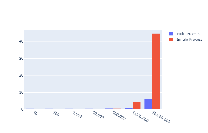
Single vs Multiprocessing for increasing simulation size

Early on in the exponentially increasing simulation size, the overhead of creating the Pool, asking the os for CPU count the splitting the attempts up to the pool seemed to result in a floor of 0.4s. However, at that level the Pi value returned was nonsense anyway. So I think the overhead for any reasonable approximation of Pi is worth the set up cost in this case.

Baby, can I get your Numba?

Can we go even further? I think we could give Numba a try.

After some research and reading around the internet for a day or so while avoiding Covid-19 I found out it is incredibly simple.

4 little chars that change everything. @jit

from random import random
from numba import njit, jit

@jit
def calc_pi_numba(num_attempts: int) -> float:
    inside = 0

    for _ in range(num_attempts):
        x = random()
        y = random()

        if x ** 2 + y ** 2 <= 1:
            inside += 1

    return 4 * inside / num_attempts

That is it. Just one import and one teensy little decorator and we are away. How does this stack up agianst my mighty multi monte carlo from earlier though?

Lets get some timings

import calcpi
from timeit import default_timer as timer
from datetime import timedelta
import matplotlib.pyplot as plt
import plotly.graph_objects as go

if __name__ == '__main__':
    
    num_attempts = [50, 500, 5_000, 50_000, 500_000, 5_000_000, 50_000_000]
    function_list = [calcpi.calc_pi_quick, calcpi.calc_pi_numba, calcpi.multi_calc_pi]
    results_dict = {}

    for func in function_list:

        timings = []
        
        for x in num_attempts:
        
            start = timer()
            pi = func(x)
            end = timer()  
            timings.append((end-start))
            # print("{} => Pi: {} Attempts: {} Time: {}".format(func.__name__, pi, x, timedelta(seconds=end-start)))

        results_dict[func.__name__] = timings
    
    go_data = []
    # lets pretty this up so the axis label is more readable
    x_axis = ['{:,}'.format(x) for x in num_attempts]
    
    for func in function_list:
    
        plt.plot(num_attempts, results_dict[func.__name__])
        
        go_data.append(go.Bar(name=func.__name__, x=x_axis, y=results_dict[func.__name__]))

    plt.show()

    fig = go.Figure(data=go_data)
    # Change the bar mode
    fig.update_layout(xaxis_type='category',barmode='group')
    fig.show()
        

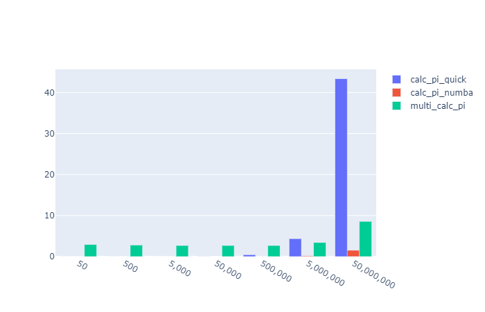
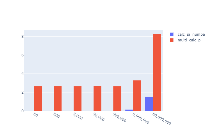
Results visulisation

X: Attempts Y: Seconds to run

Oh… it absolutely smashes it.

Out of the park for

  • Speed
  • Readability
  • Implementation simplicity

Calculate Pi using MonteCarlo Simulation – Phase I


Context

I was interviewing for a Python developer role in an Investment bank, and a nice enough but over zealous quant started asking me silly questions. You know the sort. However in this case I didnt really know the answer. So I have determined to provide a solution I am happy that I understand and also at the same time gets me into new areas of Python development.

Question:

How would calculate the value of Pi, from scratch / first principles?

Answer I gave:

“Uhhh, pardon?

Answer I should have given:

The equation for a circle is (x-h)2 + (y-k)2 = r2. With the centre as the origin and a radius of 1 we can cancel out to : x2 + y2 ≤ 1

We then look at a quarter of the circle to take away a lot of the maths needed, and randomly insert points into the resulting square. The random, co-ords are known to be either inside or outside of the desired area. We then can get the estimation of Pi as :

We know that (Points in the circle)/(Total points) = (πr2)/(2*r)2

Which we can solve for a radius of 1 as (Points in the circle)/(Total points) = (π)/(2)2

Then π = 4 * (Points in the circle)/(Total points)

Python Implementation

Err… ok. I feel now this was quite spurious in an interview situation, but lets look at the python and see what we can do.

def calc_pi(num_attempts, display_plot=False):

    import matplotlib
    import matplotlib.pyplot as plt
    from random import random
    
    inside = 0

    x_inside = []
    y_inside = []
    x_outside = []
    y_outside = []

    for _ in range(num_attempts):
        x = random()
        y = random()
        if x**2+y**2 <= 1:
            inside += 1
            x_inside.append(x)
            y_inside.append(y)
        else:
            x_outside.append(x)
            y_outside.append(y)

    pi = 4*inside/num_attempts
    
    if display_plot:
        fig, ax = plt.subplots()
        ax.set_aspect('equal')
        ax.scatter(x_inside, y_inside, color='g')
        ax.scatter(x_outside, y_outside, color='r')

    return pi
Attempting Monte Carlo Simulation with 50 attempts. 
Pi: 3.28 

Attempting Monte Carlo Simulation with 500 attempts. 
Pi: 2.992 

Attempting Monte Carlo Simulation with 5000 attempts. 
Pi: 3.176 

Attempting Monte Carlo Simulation with 50000 attempts. 
Pi: 3.14688 

Real PI: 3.141592653589793

Plotly Visualisation

Continuing with this “interview answer” level of solution, this might make for a cool Jupyter Notebook. Lets get a graphical representation.

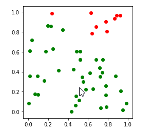
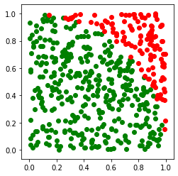
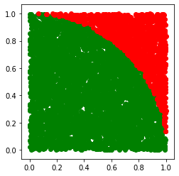
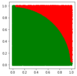
Lo and behold, it does! Trying with ever increasing attempts shows the quarter circle becoming more and more clear.

Monte Carlo Simulation with 50 attempts. Pi: 3.28
Monte Carlo Simulation with 500 attempts. Pi: 2.992
Monte Carlo Simulation with 5000 attempts. Pi: 3.176
Monte Carlo Simulation with 50000 attempts. Pi: 3.14688

Run Multiple times to get a mean average?

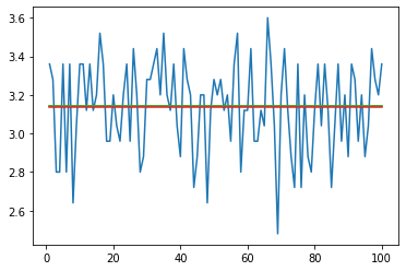
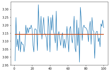
I thought that with low numbers there would be quite a large variance but the mean over multiple times would still be decent.

def plot_attempt_pi_MC_n_times(num_times, mc_attempts):

    # ok, lets use this function to try to see what the drift between that and Pi is.
    import matplotlib.pyplot as plt
    import statistics

    pi_vals = []

    for i in range(num_times):
        pi = calc_pi(mc_attempts)
        pi_vals.append(pi)

    attempt = list(range(1, num_times + 1))
    actual_pi = [math.pi]*num_times

    plt.plot(attempt, pi_vals)
    plt.plot(attempt, actual_pi)
    # a really simple arithmetic way of getting pretty close
    plt.plot(attempt, [22/7]*num_times)
    avg = statistics.mean(pi_vals)
    
    plt.plot(attempt, [avg]*num_times)
    print('Avg: {}. Diff to actual Pi: {}'.format(avg, abs(math.pi - avg)))
    plt.show()
    return pi_vals

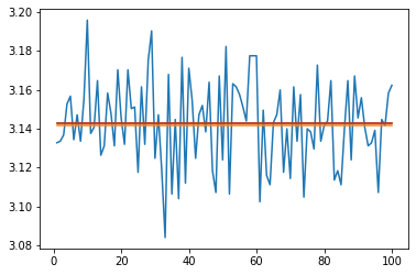
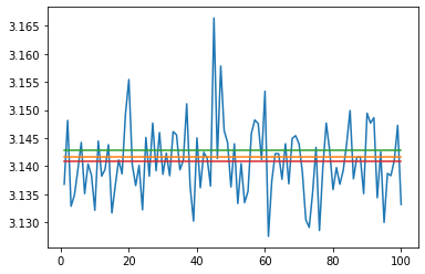
So we can multiple times, and plot each result, then take the mean compared to the same number of attempts in one single Monte Carlo evaluation

Code to try both versions of the same number of paths

mc_pi = calc_pi(5000)
print('calc_pi(5000): {}. Diff to actual Pi: {}'.format(mc_pi, abs(math.pi - mc_pi)))
w = plot_attempt_pi_MC_n_times(100, 50)

mc_pi = calc_pi(50_000)
print('calc_pi(50_000): {}. Diff to actual Pi: {}'.format(mc_pi, abs(math.pi - mc_pi)))
x = plot_attempt_pi_MC_n_times(100, 500)

mc_pi = calc_pi(500_000)
print('calc_pi(500_000): {}. Diff to actual Pi: {}'.format(mc_pi, abs(math.pi - mc_pi)))
y = plot_attempt_pi_MC_n_times(100, 5_000)

mc_pi = calc_pi(5_000_000)
print('calc_pi((5_000_000): {}. Diff to actual Pi: {}'.format(mc_pi, abs(math.pi - mc_pi)))
z = plot_attempt_pi_MC_n_times(100, 50_000)

5,000 Attempts

calc_pi(5000): 3.1376. Diff to actual Pi: 0.003992653589793171
Avg: 3.136. Diff to actual Pi: 0.005592653589792995

50,000 Attempts

calc_pi(50_000): 3.14408. Diff to actual Pi: 0.002487346410207092
Avg: 3.14256. Diff to actual Pi: 0.000967346410206904

500,000 Attempts

calc_pi(500_000): 3.144032. Diff to actual Pi: 0.002439346410207044
Avg: 3.14292. Diff to actual Pi: 0.001327346410207042

5,000,000 Attempts

calc_pi((5_000_000): 3.1420616.
Diff to actual Pi: 0.00046894641020678307
Avg: 3.1408424.
Diff to actual Pi: 0.0007502535897931928

Conclusion

We can say without a doubt that this method of calculating Pi is both expensive AND inncaurate compared to even 22/7. This approximation only gets beaten after millions of simulation steps.

It was however an interesting foray into a number of areas of maths and Python. While it is a bit mad I would like to keep going with this. How can we make this faster locally, and what it we turned to alternative solutions like the power of the cloud to get within .. say a reliable 10dp?

Follow-up

CALCULATE PI USING MONTECARLO SIMULATION – PHASE II

Excel VBA Interview questions


I started this blog mainly to record my experiences while looking for Excel / VBA roles.   I do remember that there were a number of blogs that I myself found very useful.  This one always stick in my mind as I remember using 2 posts on the blog for both my current spate of job hunting and also the previous spate where I first started to look for Excel / VBA / RAD roles when I worked out I just wasn’t going to make a very good C++ programmer.

Excel VBA Questions:

http://www.toomik.net/helen/blog/2007/01/31/interviewing-for-an-excel-vba-job/

Hiring:

http://www.toomik.net/helen/blog/2006/02/28/hiring/

I’ll post some more thoughts up on a re-edit, I just thought  I would post this up right now in my lunch break first.

New Contract!


I have managed to leave my perm employer and start in my very first contract!   I will be blogging the experience of searching, finding jobs and then interviewing for them here. 

I’ll try to get a proper blog about interview questions for :

  • Excel
  • VBA
  • Finance
  • Some C# / .Net resources
  • C++ ( not so much )

I’ll also blog about my experiences of goign contracting with a view to setting up a Limited Company, Pay schemes and Agency negotiations too.

Blog at WordPress.com.

Up ↑