
Context
I was interviewing for a Python developer role in an Investment bank, and a nice enough but over zealous quant started asking me silly questions. You know the sort. However in this case I didnt really know the answer. So I have determined to provide a solution I am happy that I understand and also at the same time gets me into new areas of Python development.
Question:
“How would calculate the value of Pi, from scratch / first principles?“
Answer I gave:
“Uhhh, pardon?“
Answer I should have given:
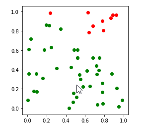
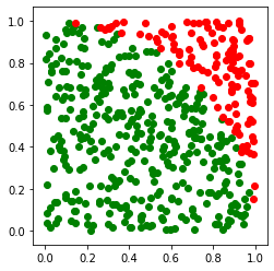
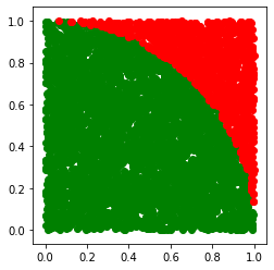
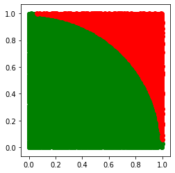
The equation for a circle is (x-h)2 + (y-k)2 = r2. With the centre as the origin and a radius of 1 we can cancel out to : x2 + y2 ≤ 1
We then look at a quarter of the circle to take away a lot of the maths needed, and randomly insert points into the resulting square. The random, co-ords are known to be either inside or outside of the desired area. We then can get the estimation of Pi as :
We know that (Points in the circle)/(Total points) = (πr2)/(2*r)2
Which we can solve for a radius of 1 as (Points in the circle)/(Total points) = (π)/(2)2
Then π = 4 * (Points in the circle)/(Total points)
Python Implementation
Err… ok. I feel now this was quite spurious in an interview situation, but lets look at the python and see what we can do.
def calc_pi(num_attempts, display_plot=False):

    import matplotlib
    import matplotlib.pyplot as plt
    from random import random

    inside = 0

    x_inside = []
    y_inside = []
    x_outside = []
    y_outside = []

    for _ in range(num_attempts):
        x = random()
        y = random()
        if x**2+y**2 <= 1:
            inside += 1
            x_inside.append(x)
            y_inside.append(y)
        else:
            x_outside.append(x)
            y_outside.append(y)

    pi = 4*inside/num_attempts

    if display_plot:
        fig, ax = plt.subplots()
        ax.set_aspect('equal')
        ax.scatter(x_inside, y_inside, color='g')
        ax.scatter(x_outside, y_outside, color='r')

    return pi
Attempting Monte Carlo Simulation with 50 attempts.
Pi: 3.28

Attempting Monte Carlo Simulation with 500 attempts.
Pi: 2.992

Attempting Monte Carlo Simulation with 5000 attempts.
Pi: 3.176

Attempting Monte Carlo Simulation with 50000 attempts.
Pi: 3.14688

Real PI: 3.141592653589793
Plotly Visualisation
Continuing with this “interview answer” level of solution, this might make for a cool Jupyter Notebook. Lets get a graphical representation.
Lo and behold, it does! Trying with ever increasing attempts shows the quarter circle becoming more and more clear.
Run Multiple times to get a mean average?
I thought that with low numbers there would be quite a large variance but the mean over multiple times would still be decent.
def plot_attempt_pi_MC_n_times(num_times, mc_attempts):

    # ok, lets use this function to try to see what the drift between that and Pi is.
    import matplotlib.pyplot as plt
    import statistics

    pi_vals = []

    for i in range(num_times):
        pi = calc_pi(mc_attempts)
        pi_vals.append(pi)

    attempt = list(range(1, num_times + 1))
    actual_pi = [math.pi]*num_times

    plt.plot(attempt, pi_vals)
    plt.plot(attempt, actual_pi)
    # a really simple arithmetic way of getting pretty close
    plt.plot(attempt, [22/7]*num_times)
    avg = statistics.mean(pi_vals)

    plt.plot(attempt, [avg]*num_times)
    print('Avg: {}. Diff to actual Pi: {}'.format(avg, abs(math.pi - avg)))
    plt.show()
    return pi_vals
So we can multiple times, and plot each result, then take the mean compared to the same number of attempts in one single Monte Carlo evaluation
Code to try both versions of the same number of paths
mc_pi = calc_pi(5000)
print('calc_pi(5000): {}. Diff to actual Pi: {}'.format(mc_pi, abs(math.pi - mc_pi)))
w = plot_attempt_pi_MC_n_times(100, 50)

mc_pi = calc_pi(50_000)
print('calc_pi(50_000): {}. Diff to actual Pi: {}'.format(mc_pi, abs(math.pi - mc_pi)))
x = plot_attempt_pi_MC_n_times(100, 500)

mc_pi = calc_pi(500_000)
print('calc_pi(500_000): {}. Diff to actual Pi: {}'.format(mc_pi, abs(math.pi - mc_pi)))
y = plot_attempt_pi_MC_n_times(100, 5_000)

mc_pi = calc_pi(5_000_000)
print('calc_pi((5_000_000): {}. Diff to actual Pi: {}'.format(mc_pi, abs(math.pi - mc_pi)))
z = plot_attempt_pi_MC_n_times(100, 50_000)
5,000 Attempts
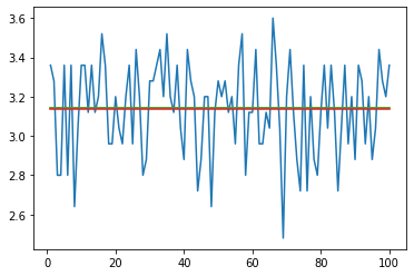
Avg: 3.136. Diff to actual Pi: 0.005592653589792995
50,000 Attempts
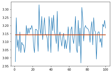
Avg: 3.14256. Diff to actual Pi: 0.000967346410206904
500,000 Attempts
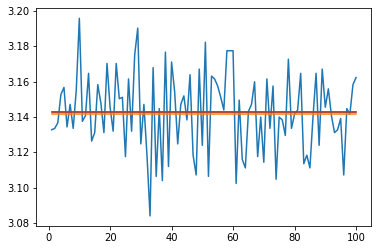
Avg: 3.14292. Diff to actual Pi: 0.001327346410207042
5,000,000 Attempts
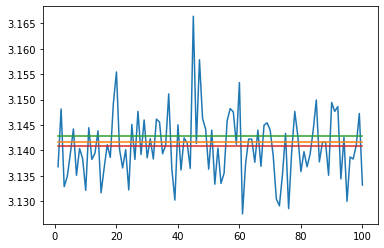
Diff to actual Pi: 0.00046894641020678307
Avg: 3.1408424.
Diff to actual Pi: 0.0007502535897931928
Conclusion
We can say without a doubt that this method of calculating Pi is both expensive AND inncaurate compared to even 22/7. This approximation only gets beaten after millions of simulation steps.
It was however an interesting foray into a number of areas of maths and Python. While it is a bit mad I would like to keep going with this. How can we make this faster locally, and what it we turned to alternative solutions like the power of the cloud to get within .. say a reliable 10dp?
