CALCULATE PI USING MONTECARLO SIMULATION – PHASE III – aka "Multicarlo"


Introduction

After Phase II, we discovered that Numpy wasn’t going to help. Also, getting a half way decent approximation of Pi was going to take millions of paths / attempts. So on a slimmed down calculation where the [x,y] position of each random try was not kept, what could be done to make this as quick and accurate as possible?

Multi-Processing?

Can I use the 16 Cores on my machine to go 16X faster? Am I being naiive here? If I am, how and what is the most that can be done? I would like to see if the infamous G.I.L will Get me Into Logjam or not.

First Attempt [Disaster]

from multiprocessing import Pool
import os

num_cpus = os.cpu_count()
print('Num of CPUS: {}'.format(num_cpus))

try:
    pool = Pool(num_cpus) # on 8 processors
    data_outputs = pool.map(calc_pi_quick, [10])
    print (data_outputs)
finally: # To make sure processes are closed in the end, even if errors happen
    pool.close()
    pool.join()

Disappointingly, not only is it not any quicker; in fact, doesn’t finish running AT ALL.

Awkward, lets look at why that is happening first?

  • I quite like Medium Articles and this one seems to hit the spot.
  • Also this from StackOverflow

Second Attempt

from random import random

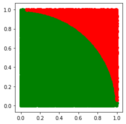
def calc_pi_quick(num_attempts: int) -> float:
    from random import random

    inside = 0

    for _ in range(num_attempts):
        x = random()
        y = random()

        if x ** 2 + y ** 2 <= 1:
            inside += 1

    return 4 * inside / num_attempts


def multi_calc_pi(num_attempts: int, verbose=False) -> float:
    from multiprocessing import Pool
    from random import random
    import os
    from statistics import mean

    # lets leave one spare for OS related things so everything doesn't freeze up
    num_cpus = os.cpu_count() - 1
    # print('Num of CPUS: {}'.format(num_cpus))

    try:
        attempts_to_try_in_process = int(num_attempts / num_cpus)
        pool = Pool(num_cpus)
        # what I am trying to do here is get the calc happening over n-1 Cpus each with an even
        # split of the num_attempts. i.e. 150 attempts over 15 CPU will lead to 10 each then the mean avg
        # of the returned list being returned.
        data_outputs = pool.map(calc_pi_quick, [attempts_to_try_in_process] * num_cpus)
        return mean(data_outputs)
    finally:  # To make sure processes are closed in the end, even if errors happen
        pool.close()
        pool.join()

To get multiprocessing to work on Jupyter Notebooks and Windows 10, I had to save this code to a different file to be called from the Jupyter Notebook, and executed within __main__. However once I did, this did lead to a significant performance increase.

Collect the Stats

import calcpi
from timeit import default_timer as timer
from datetime import timedelta
import matplotlib.pyplot as plt

if __name__ == '__main__':
    
    num_attempts = [50, 500, 5_000, 50_000, 500_000, 5_000_000, 50_000_000]
    multi_timings = []
    single_timings = []
    
    for x in num_attempts:
    
        start = timer()
        multi_pi = calcpi.multi_calc_pi(x)
        end = timer()  
        multi_timings.append((end-start))
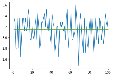
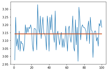
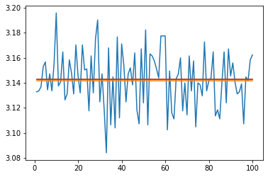
        print("MultiCarlo Pi: {}: {} took {}".format(multi_pi, x, timedelta(seconds=end-start)))

        start = timer()    
        pi = calcpi.calc_pi_quick(x)
        end = timer()
        single_timings.append((end-start))
        print("MonteCarlo Pi: {}: {} took {}".format(pi, x, timedelta(seconds=end-start)))

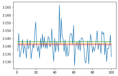
    plt.plot(num_attempts, multi_timings)
    plt.plot(num_attempts, single_timings)

    plt.show()

Display the stats in a more meaningful way

import plotly.graph_objects as go

import numpy as np

# lets pretty this up so the axis label is more readable
x_axis = ['{:,}'.format(x) for x in num_attempts]

fig = go.Figure(data=[
    go.Bar(name='Multi Process', x=x_axis, y=multi_timings),
    go.Bar(name='Single Process', x=x_axis, y=single_timings)
])
# Change the bar mode
fig.update_layout(xaxis_type='category',barmode='group')
fig.show()
Single vs Multiprocessing for increasing simulation size

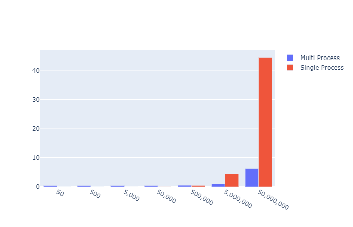
Early on in the exponentially increasing simulation size, the overhead of creating the Pool, asking the os for CPU count the splitting the attempts up to the pool seemed to result in a floor of 0.4s. However, at that level the Pi value returned was nonsense anyway. So I think the overhead for any reasonable approximation of Pi is worth the set up cost in this case.

Baby, can I get your Numba?

Can we go even further? I think we could give Numba a try.

After some research and reading around the internet for a day or so while avoiding Covid-19 I found out it is incredibly simple.

4 little chars that change everything. @jit

from random import random
from numba import njit, jit

@jit
def calc_pi_numba(num_attempts: int) -> float:
    inside = 0

    for _ in range(num_attempts):
        x = random()
        y = random()

        if x ** 2 + y ** 2 <= 1:
            inside += 1

    return 4 * inside / num_attempts

That is it. Just one import and one teensy little decorator and we are away. How does this stack up agianst my mighty multi monte carlo from earlier though?

Lets get some timings

import calcpi
from timeit import default_timer as timer
from datetime import timedelta
import matplotlib.pyplot as plt
import plotly.graph_objects as go

if __name__ == '__main__':
    
    num_attempts = [50, 500, 5_000, 50_000, 500_000, 5_000_000, 50_000_000]
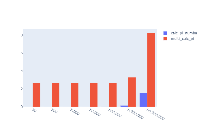
    function_list = [calcpi.calc_pi_quick, calcpi.calc_pi_numba, calcpi.multi_calc_pi]
    results_dict = {}

    for func in function_list:

        timings = []
        
        for x in num_attempts:
        
            start = timer()
            pi = func(x)
            end = timer()  
            timings.append((end-start))
            # print("{} => Pi: {} Attempts: {} Time: {}".format(func.__name__, pi, x, timedelta(seconds=end-start)))

        results_dict[func.__name__] = timings
    
    go_data = []
    # lets pretty this up so the axis label is more readable
    x_axis = ['{:,}'.format(x) for x in num_attempts]
    
    for func in function_list:
    
        plt.plot(num_attempts, results_dict[func.__name__])
        
        go_data.append(go.Bar(name=func.__name__, x=x_axis, y=results_dict[func.__name__]))

    plt.show()

    fig = go.Figure(data=go_data)
    # Change the bar mode
    fig.update_layout(xaxis_type='category',barmode='group')
    fig.show()
        

Results visulisation

X: Attempts Y: Seconds to run

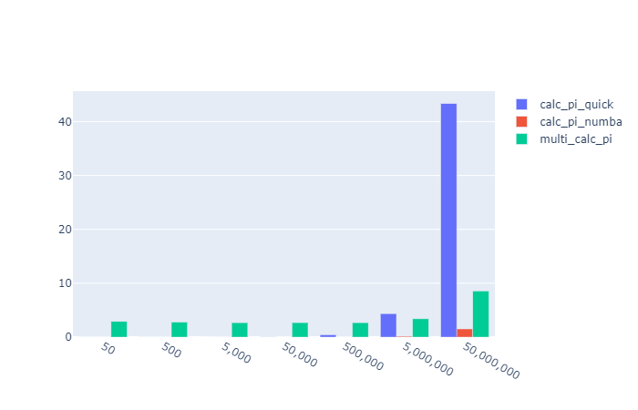
Oh… it absolutely smashes it.

Out of the park for

  • Speed
  • Readability
  • Implementation simplicity

CALCULATE PI USING MONTECARLO SIMULATION – PHASE II


Context

Carrying on from Phase I, I wanted to see how I could take the initial answer and make it more efficient. The first port of call then is… how expensive is it at the moment. Will any changes I make have a significant impact on that baseline.

timeit

I dont think using %%timeit as an ipython coding secret on the cell will cut the mustard, but we shall see. I would like to be able to single out code sections for timing too.

Calc Pi Unoptimised

def calc_pi(num_attempts, display_plot=False):

    import matplotlib
    import matplotlib.pyplot as plt
    from random import random
    
    inside = 0

    x_inside = []
    y_inside = []
    x_outside = []
    y_outside = []

    for _ in range(num_attempts):
        x = random()
        y = random()
        if x**2+y**2 <= 1:
            inside += 1
            x_inside.append(x)
            y_inside.append(y)
        else:
            x_outside.append(x)
            y_outside.append(y)

    pi = 4*inside/num_attempts
    
    if display_plot:
        fig, ax = plt.subplots()
        ax.set_aspect('equal')
        ax.scatter(x_inside, y_inside, color='g')
        ax.scatter(x_outside, y_outside, color='r')

    return pi

Calc Pi Quick (Version 1)

Quick Python only changes, remove array recording and if we never plan to plot remove the if statement

def calc_pi_quick(num_attempts: int):

    inside = 0

    for _ in range(num_attempts):
        x = random()
        y = random()
        if x**2+y**2 <= 1:
            inside += 1

    return 4*inside/num_attempts

Initial comparison

from timeit import default_timer as timer
from datetime import timedelta

start = timer()
calc_pi(50000000, True)
end = timer()
print(timedelta(seconds=end-start))

start = timer()
calc_pi(50000000, False)
end = timer()
print(timedelta(seconds=end-start))

start = timer()
calc_pi_quick(50000000)
end = timer()
print(timedelta(seconds=end-start))

Output

calc_pi with plotly display time: 0:00:08.318734 
calc_pi no display time: 0:00:00.625193 
calc_pi_quick time: 0:00:00.470770

We start to see there are some decent performance benefits. Lets check if these are linear or not. However to see some really decent improvements I think we can start to think about threading perhaps? Also if we still wanted to record the hit and miss positions, would numpy be quick enough that we can keep this data without a significant performance hit?

Numpy Optimisation Attempts

Spoiler Alert… my first attempt was absolutely terrible. However, in a way that’s great news. I now know what not to do with numpy on a non trivial problem, and now so do you.

def calc_pi_numpi_bad(num_attempts):
    
    import numpy as np
    import matplotlib
    import matplotlib.pyplot as plt
    from random import random
    
    inside = 0

    x_inside = np.array([])
    y_inside = np.array([])
    x_outside = np.array([])
    y_outside = np.array([])

    for _ in range(num_attempts):
        x = random()
        y = random()
        if x**2+y**2 <= 1:
            inside += 1
            x_inside = np.append(x_inside, x)
            y_inside = np.append(y_inside, y)
        else:
            x_outside = np.append(x_outside, x)
            y_outside = np.append(y_outside, y)

    pi = 4*inside/num_attempts

    return pi

How bad? Well lets see…

def measure_performance_verbose(num_attempts: int) -> None:

    from timeit import default_timer as timer
    from datetime import timedelta

    start = timer()
    calc_pi(num_attempts, False)
    end = timer()
    time_taken = end-start
    print('calc_pi time: {}'.format(timedelta(seconds=time_taken)))

    start = timer()
    calc_pi_quick(num_attempts)
    end = timer()
    quick_time_taken = end-start
    print('calc_pi_quick time: {}'.format(timedelta(seconds=quick_time_taken)))

    percentage_improvement = quick_time_taken / time_taken * 100
    
    print('Precentage improvement: {}'.format(percentage_improvement))

    start = timer()
    calc_pi_numpi(num_attempts)
    end = timer()
    numpi_time_taken = end-start
    print('calc_pi_numpi time: {}'.format(timedelta(seconds=numpi_time_taken)))
    
    start = timer()
    calc_pi_numpi_bad(num_attempts)
    end = timer()
    numpi_bad_time_taken = end-start
    print('calc_pi_numpi_bad time: {}'.format(timedelta(seconds=numpi_bad_time_taken)))
    
    
measure_performance_verbose(500_000)
calc_pi time: 0:00:00.636658
calc_pi_quick time: 0:00:00.462309
Precentage improvement: 72.6149660351135
calc_pi_numpi time: 0:00:00.616958
calc_pi_numpi_bad time: 0:12:52.784511

Whoa, what just happened there. It takes TWELVE seconds to run for 500,000 attempts. That is atrocious.

Lets look at the documentation for this function.

Ahh, that explains it. Every append copies the existing array into a new one. I did not know that, shame on me. I have always used np arrays as data converted from pandas or existing python lists, not created and appended to them on the fly.

However, we can fix it by pre-allocating the mem to the max num required and then mask the results if zero in plotly.

def calc_pi_numpi(num_attempts, display_plot=False, display_masked_plot=False):
    
    import numpy as np
    import matplotlib
    import matplotlib.pyplot as plt
    from random import random
    
    inside = 0

    x_inside = np.zeros(num_attempts)
    y_inside = np.zeros(num_attempts)
    x_outside = np.zeros(num_attempts)
    y_outside = np.zeros(num_attempts)

    for i in range(num_attempts):
        x = random()
        y = random()
        if x**2+y**2 <= 1:
            inside += 1
            x_inside[i] = x
            y_inside[i] = y
        else:
            x_outside[i] = x
            y_outside[i] = y

    if display_masked_plot:
        
        fig, ax = plt.subplots()
        ax.set_aspect('equal')
        ax.scatter(np.ma.masked_equal(x_inside,0), np.ma.masked_equal(y_inside,0), color='g')
        ax.scatter(np.ma.masked_equal(x_outside,0), np.ma.masked_equal(y_outside,0), color='r')
        
    if display_plot:
            
        x_inside2 = x_inside[x_inside !=0] 
        y_inside2 = y_inside[y_inside !=0]
        x_outside2 = x_outside[x_outside !=0]
        y_outside2 = y_outside[y_outside !=0]

        fig, ax = plt.subplots()
        ax.set_aspect('equal')
        ax.scatter(x_inside2, y_inside2, color='g')
        ax.scatter(x_outside2, y_outside2, color='r')

    pi = 4*inside/num_attempts

    return pi

There are two booleans so that we can test that both work.

calc_pi_numpi(256, True, True)
masked


numpy zero removal
start = timer()
calc_pi_numpi(500_000, True, False)
end = timer()
time_taken = end-start
print('calc_pi normal display time: {}'.format(timedelta(seconds=time_taken)))

start = timer()
calc_pi_numpi(500_000, False, True)
end = timer()
time_taken = end-start
print('calc_pi masked display time: {}'.format(timedelta(seconds=time_taken)))
calc_pi normal display time: 0:00:02.356013
calc_pi masked display time: 0:00:04.012019

Much much better.

start = timer()
calc_pi_numpi(500_000, False, False)
end = timer()
time_taken = end-start
print('calc_pi no display time: {}'.format(timedelta(seconds=time_taken)))

start = timer()
calc_pi(500_000)
end = timer()
time_taken = end-start
print('calc_pi no display time: {}'.format(timedelta(seconds=time_taken)))
calc_pi no display time: 0:00:00.622075 
calc_pi no display time: 0:00:00.655379

So… numpy doesn’t make things better, but used correctly, doesn’t make things any worse. So this is a dead end. Also we don’t want to plot for the numbers higher than a million as it looks to the human eye to be , a complete quarter circle. in plotly anyway so we dont need to store large amounts of array data anyway

While I am here I wanted to utilise the “functions are first class objects” paradigm in python. I have hinted at it by showing the initial fuction as _verbose but its much cleaner to call that same code within a functor ( of sorts ) loop as below.

def measure_performance(num_attempts: int) -> None:

    from timeit import default_timer as timer
    from datetime import timedelta
    
    funcs_to_call = [calc_pi, calc_pi_quick, calc_pi_numpi, calc_pi_numpi_bad]
    
    for func in funcs_to_call:
        start = timer()
        calc_pi(num_attempts, False)
        end = timer()
        time_taken = end-start
        print('{} time: {}'.format(func.__name__, timedelta(seconds=time_taken)))
    
measure_performance(50000)

In Phase III -> aka PiMultiCarlo I want to loo at what we can do locally on a decent multi core machine to get some decent speed improvements for only calculating the number only, not storing the guesses.

Follow-up

For Part III : CALCULATE PI USING MONTECARLO SIMULATION – PHASE III – aka “Multicarlo”

Calculate Pi using MonteCarlo Simulation – Phase I


Context

I was interviewing for a Python developer role in an Investment bank, and a nice enough but over zealous quant started asking me silly questions. You know the sort. However in this case I didnt really know the answer. So I have determined to provide a solution I am happy that I understand and also at the same time gets me into new areas of Python development.

Question:

How would calculate the value of Pi, from scratch / first principles?

Answer I gave:

“Uhhh, pardon?

Answer I should have given:

The equation for a circle is (x-h)2 + (y-k)2 = r2. With the centre as the origin and a radius of 1 we can cancel out to : x2 + y2 ≤ 1

We then look at a quarter of the circle to take away a lot of the maths needed, and randomly insert points into the resulting square. The random, co-ords are known to be either inside or outside of the desired area. We then can get the estimation of Pi as :

We know that (Points in the circle)/(Total points) = (πr2)/(2*r)2

Which we can solve for a radius of 1 as (Points in the circle)/(Total points) = (π)/(2)2

Then π = 4 * (Points in the circle)/(Total points)

Python Implementation

Err… ok. I feel now this was quite spurious in an interview situation, but lets look at the python and see what we can do.

def calc_pi(num_attempts, display_plot=False):

    import matplotlib
    import matplotlib.pyplot as plt
    from random import random
    
    inside = 0

    x_inside = []
    y_inside = []
    x_outside = []
    y_outside = []

    for _ in range(num_attempts):
        x = random()
        y = random()
        if x**2+y**2 <= 1:
            inside += 1
            x_inside.append(x)
            y_inside.append(y)
        else:
            x_outside.append(x)
            y_outside.append(y)

    pi = 4*inside/num_attempts
    
    if display_plot:
        fig, ax = plt.subplots()
        ax.set_aspect('equal')
        ax.scatter(x_inside, y_inside, color='g')
        ax.scatter(x_outside, y_outside, color='r')

    return pi
Attempting Monte Carlo Simulation with 50 attempts. 
Pi: 3.28 

Attempting Monte Carlo Simulation with 500 attempts. 
Pi: 2.992 

Attempting Monte Carlo Simulation with 5000 attempts. 
Pi: 3.176 

Attempting Monte Carlo Simulation with 50000 attempts. 
Pi: 3.14688 

Real PI: 3.141592653589793

Plotly Visualisation

Continuing with this “interview answer” level of solution, this might make for a cool Jupyter Notebook. Lets get a graphical representation.

Lo and behold, it does! Trying with ever increasing attempts shows the quarter circle becoming more and more clear.

Monte Carlo Simulation with 50 attempts. Pi: 3.28
Monte Carlo Simulation with 500 attempts. Pi: 2.992
Monte Carlo Simulation with 5000 attempts. Pi: 3.176
Monte Carlo Simulation with 50000 attempts. Pi: 3.14688

Run Multiple times to get a mean average?

I thought that with low numbers there would be quite a large variance but the mean over multiple times would still be decent.

def plot_attempt_pi_MC_n_times(num_times, mc_attempts):

    # ok, lets use this function to try to see what the drift between that and Pi is.
    import matplotlib.pyplot as plt
    import statistics

    pi_vals = []

    for i in range(num_times):
        pi = calc_pi(mc_attempts)
        pi_vals.append(pi)

    attempt = list(range(1, num_times + 1))
    actual_pi = [math.pi]*num_times

    plt.plot(attempt, pi_vals)
    plt.plot(attempt, actual_pi)
    # a really simple arithmetic way of getting pretty close
    plt.plot(attempt, [22/7]*num_times)
    avg = statistics.mean(pi_vals)
    
    plt.plot(attempt, [avg]*num_times)
    print('Avg: {}. Diff to actual Pi: {}'.format(avg, abs(math.pi - avg)))
    plt.show()
    return pi_vals

So we can multiple times, and plot each result, then take the mean compared to the same number of attempts in one single Monte Carlo evaluation

Code to try both versions of the same number of paths

mc_pi = calc_pi(5000)
print('calc_pi(5000): {}. Diff to actual Pi: {}'.format(mc_pi, abs(math.pi - mc_pi)))
w = plot_attempt_pi_MC_n_times(100, 50)

mc_pi = calc_pi(50_000)
print('calc_pi(50_000): {}. Diff to actual Pi: {}'.format(mc_pi, abs(math.pi - mc_pi)))
x = plot_attempt_pi_MC_n_times(100, 500)

mc_pi = calc_pi(500_000)
print('calc_pi(500_000): {}. Diff to actual Pi: {}'.format(mc_pi, abs(math.pi - mc_pi)))
y = plot_attempt_pi_MC_n_times(100, 5_000)

mc_pi = calc_pi(5_000_000)
print('calc_pi((5_000_000): {}. Diff to actual Pi: {}'.format(mc_pi, abs(math.pi - mc_pi)))
z = plot_attempt_pi_MC_n_times(100, 50_000)

5,000 Attempts

calc_pi(5000): 3.1376. Diff to actual Pi: 0.003992653589793171
Avg: 3.136. Diff to actual Pi: 0.005592653589792995

50,000 Attempts

calc_pi(50_000): 3.14408. Diff to actual Pi: 0.002487346410207092
Avg: 3.14256. Diff to actual Pi: 0.000967346410206904

500,000 Attempts

calc_pi(500_000): 3.144032. Diff to actual Pi: 0.002439346410207044
Avg: 3.14292. Diff to actual Pi: 0.001327346410207042

5,000,000 Attempts

calc_pi((5_000_000): 3.1420616.
Diff to actual Pi: 0.00046894641020678307
Avg: 3.1408424.
Diff to actual Pi: 0.0007502535897931928

Conclusion

We can say without a doubt that this method of calculating Pi is both expensive AND inncaurate compared to even 22/7. This approximation only gets beaten after millions of simulation steps.

It was however an interesting foray into a number of areas of maths and Python. While it is a bit mad I would like to keep going with this. How can we make this faster locally, and what it we turned to alternative solutions like the power of the cloud to get within .. say a reliable 10dp?

Follow-up

CALCULATE PI USING MONTECARLO SIMULATION – PHASE II

Blog at WordPress.com.

Up ↑